Neurorack

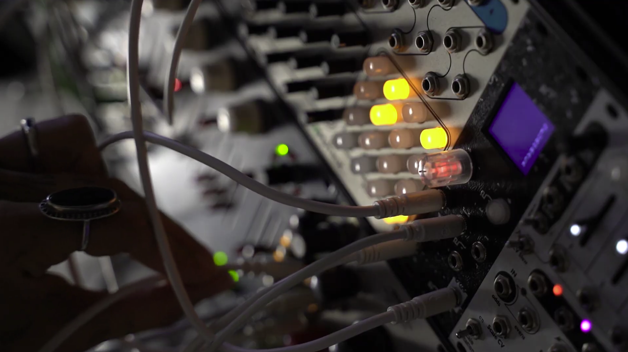
The Neurorack is a Eurorack module with a deep generative model running on embedded hardware inside it, playing as an ordinary rack voice. It was built in the ACIDS group at IRCAM during my doctorate, and has been rebuilt and extended since, most recently for a live set at Berghain’s Säule.

This page describes the instrument as it currently stands: how it generates sound, what the panel does, and the design constraints that shaped both. The 2022 paper below describes the original system.

---

A generative model inside a 23 millisecond deadline

Most of the engineering follows from one number. The audio process runs in blocks of 512 frames at a 22.05 kHz sample rate:

512 ⁄ 22050 Hz ≈ 23.2 ms the time available to produce one block of output

Model inference, post-model DSP and output all have to finish inside that window, every block, with no exceptions. A generative model that is merely fast on average is of no use here: a single overrun is an audible click. This is the difference between offline synthesis, where quality is bounded by patience, and an instrument, where quality is bounded by a deadline.

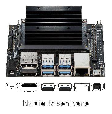
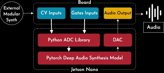
The computational core is an NVIDIA Jetson Nano (quad-core ARM, 128-core Maxwell GPU, 4 GB LPDDR4), with a PCM5102 I²S DAC, two ADS1015 ADCs on I²C for the control voltages, and an ST7789 SPI display.

Work is split across four processes, each with its own deadline:

Process	Rate	Job
audio	512 frames / 23.2 ms	model inference, post-DSP, output
cv	250 Hz	read the ADCs, condition and publish
ui	60 Hz input, 20 FPS frames	panel, screen, LED
parent	2 Hz	supervise, handle shutdown

The audio process runs at elevated priority and the interface deliberately at the lowest, so that redrawing a screen can never preempt sound. Parameter edits cross from the interface to the audio process through shared memory rather than a queue, so no interface work can block a note.

---

Synthesis: conditioning on perceptual descriptors

The model does not synthesise from an oscillator. It reconstructs a waveform from a description of one.

That description is a trajectory of seven spectral descriptors per frame, computed from the training audio and, at play time, supplied by the instrument:

Descriptor	Definition	What it controls
Loudness	RMS = √( (1/N) Σ x[n]² )	weight
Percussivity	zero-crossing rate	grain, buzz
Brightness	spectral centroid	perceived brightness
Tone	spectral roll-off	where the energy stops
Richness	spectral bandwidth	spread around the centroid
Noise	spectral flatness	tonal against noisy
Pitch	fundamental f₀	pitch

Two of these carry most of the perceptual weight. The centroid is the amplitude-weighted mean frequency of the spectrum, which is the standard correlate of perceived brightness:

centroid = ( Σ_f f · |X(f)| ) ⁄ ( Σ_f |X(f)| ) X(f) is the magnitude spectrum of the frame

Flatness is the ratio of the geometric to the arithmetic mean of the magnitude spectrum, approaching 1 for noise and 0 for a pure tone:

flatness = exp( (1/K) Σ_f ln |X(f)| ) ⁄ ( (1/K) Σ_f |X(f)| ) K is the number of frequency bins

Conditioning on descriptors rather than on raw spectral frames is the decision the whole instrument rests on. It reduces the control surface from hundreds of bins per frame to seven numbers; those seven are perceptually meaningful rather than arbitrary; and because each is a scalar, each maps directly onto a control voltage. A latent vector would be smaller still but would not have axes anyone could name, let alone patch a sequencer into.

The model

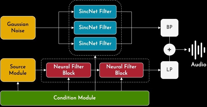
Synthesis uses an adapted Sinc-NSF (neural source-filter) model, an architecture borrowed from speech synthesis. Source-filter models separate excitation from resonance, generating a harmonic component and a noise component and shaping them with filters, in a single forward pass rather than autoregressively. That single pass is what makes the deadline above achievable.

The filters are SincNet bandpass filters, which are parameterised by their cutoff frequencies rather than by learned taps. A conventional learned FIR filter of length L carries L free parameters with no constraint on their shape; a sinc filter carries two, a low and a high cutoff, and is band-pass by construction. This is a strong structural prior: fewer parameters, faster convergence, and filters whose learned values can be read as frequencies.

Training minimises a multi-resolution spectral loss, comparing magnitude spectrograms at several window sizes at once:

ℒ = Σ_r ‖ |STFT_r(x)| − |STFT_r(x̂)| ‖ r indexes the analysis resolutions, x̂ the reconstruction

The multiple resolutions matter for this material specifically. A short window resolves the transient that makes an impact read as a strike; a long window resolves the tail that gives it a body. Optimising at one resolution alone sacrifices whichever the window is blind to. The deployed weights are an exponential moving average over training, which is noticeably steadier than the final checkpoint.

The training set was roughly 3,500 curated impact samples at 44.1 kHz, normalised and trimmed. A variational autoencoder trained on the descriptor curves provides a low-dimensional latent space from which new, coherent descriptor trajectories can be sampled rather than only replayed.

---

Three sources and a simplex

Three descriptor sets are loaded at once, in slots A, B and C, and playing the instrument largely consists of moving through the space between them.

That space is a 2-simplex, a triangle whose vertices are the three sources, and it is navigated in two coordinates. Morph is an angle θ travelling around the perimeter; Focus is a radius, blending the perimeter position toward the centroid where all three sources contribute equally. The weights are barycentric:

w = focus · w_perimeter(θ) + (1 − focus) · (1/3, 1/3, 1/3),   Σ w_i = 1 focus = 1 sits on an edge between two sources; focus = 0 sits at the centre of all three

Morph at full focus therefore interpolates between two sources at a time, while lowering focus pulls the result toward a three-way average. Because the weights always sum to one, every position in the triangle is a valid convex combination and nothing can run off the edge of the trained space.

Hybrid tails

A separate pair of controls, Hybrid Donor and Hybrid Amount, lets one descriptor set lend only the tail of its trajectory to another. The result is a strike whose body comes from one material and whose decay comes from a different one.

This cannot be reached by morphing, and the reason is structural. A morph is a weighted sum over whole trajectories, so it moves every descriptor column at once and at every point in time. A hybrid splits the time axis instead and substitutes the later frames alone. The two operations act on different axes of the same tensor, which is why the instrument exposes both.

---

A second engine

A granular voice now runs alongside the neural one, reading the same source recordings directly rather than through the model. Engine Blend crossfades between them. Both voices are triggered by the same gate and shaped by the same envelope, so any intermediate setting is two renderings of one note rather than two unrelated sounds layered together.

What makes this more than a dry/wet control is that the same panel gesture means something different in each engine. Turning Morph in the neural engine interpolates a descriptor trajectory and resynthesises from the result. Turning Morph in the granular engine draws grains from all three recordings in proportion. One is interpolation in a parameter space; the other is mixture in a sample space. The knob is the same, the mathematics is not, and the two disagree in ways that are musically useful.

Scrub selects where in a recording each grain is read from, and Variation scatters that position per grain so the texture does not freeze.

---

Latency as a design taxonomy

Because some parameters act after the model and others act on its input, they do not take effect at the same time. Rather than hide this, the instrument makes it the organising principle of the interface: every parameter carries a tier badge saying when a change will be heard.

Tier A, inside one audio block (under 25 ms). Level, Decay, Tilt, Drive, Engine Blend, Texture. These are applied to the audio after the model, so they change a note while it is sounding. An envelope or an audio-rate LFO patched here behaves exactly as it would on an analogue module.

Tier C, on the next gate. Morph, Focus, Scrub, Variation, the three source slots, Hybrid Donor and Amount, Brightness, Noisiness, Body, Detune, Transient. All of these rebuild the conditioning tensor, so the sound has to be regenerated and the change lands on the next trigger. While one is pending the screen reads ARMED, the value renders as an outline, and the LED pulses amber.

Tier B, reserved and deliberately empty (50 to 100 ms). This would be genuine per-frame descriptor streaming, modulation following an LFO smoothly through a note the way a filter cutoff does. The architecture does not support it: anything touching the conditioning tensor currently has to rebuild it whole. The tier is defined but unassigned so that a later firmware can register into it without changing the menu, the modulation matrix or the preset format.

The practical consequence is a rule a player can hold in their head. Fast modulation goes to Tier A. Sweeps you want to hear step from note to note go to Tier C. The constraint is real, and naming it turned out to be more useful than disguising it.

---

The panel

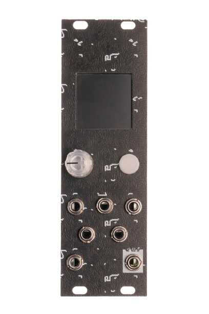
Jack / control	Type	Range
GATE 1	Gate in	trigger, +1.0 V rising / +0.6 V falling
GATE 2	Gate in	assignable, Freeze by default
CV 1–4	CV in	±5 V, assignable
OUT	Audio out	stereo DAC, 22.05 kHz
Encoder	Rotary, turn only	no push switch
Button	Momentary	the only key
Screen	240×240 colour LCD	20 FPS

Control voltages

CV 1 is pitch, one volt per octave, with optional quantisation to the nearest semitone. CV 2 to 4 can be assigned to any parameter in the instrument. Each jack carries its own conditioning chain before it reaches its destination:

• Depth, an attenuverter from −100 % to +100 %, so one modulation source can move two destinations in opposite directions
• Offset, a bias from −100 % to +100 %
• Curve, linear, exponential, logarithmic or S
• Slew, 0 to 500 ms

From the factory, CV 2 is Tilt, CV 3 is Reverb Mix and CV 4 is Engine Blend, all of them Tier A and therefore audible mid-note.

Gates

Either gate can be assigned one of nine actions, with a selectable edge (rising, falling or both) and a threshold between 0.5 V and 4.0 V:

Action	Effect
Trigger	fire a note
Retrig	restart the current note
Freeze	hold the current output
Regen	a fresh take of the current sound
Env	gate the envelope
Clock	use the gate as a time base
Step	advance one source slot
Texture	hold a sustaining texture while high
Preset	recall a stored scene

Texture is the one worth singling out. Holding the gate keeps generation running past the natural length of the source material, drifting as it goes, which gives an instrument built around impacts a sustaining register.

---

Determinism

Generation is reproducible by construction. The neural engine’s seed is derived from a signature of the conditioning tensor itself, and the granular engine’s jitter is seeded per note, so identical settings produce identical audio.

This matters twice over. In research it makes a rendered example an artefact someone else can regenerate rather than a recording they have to take on trust. On stage it means a sound found in rehearsal is still there hours later, which is the difference between an instrument and a generator of pleasant surprises.

---

Listen

A track composed entirely from impact sounds generated by the Neurorack:

---

Development

V1 proved that embedded real-time neural synthesis was possible at all, with exposed cabling, external power, a model burn-in on startup and descriptor sets fixed at compile time.

V2, with Corentin Vercoustre, Valentin Lageard and Martin Vert, internalised the wiring and redesigned the faceplate, and began the integration of FRAVE, a model built for continuous timbral control through a latent space.

The current build adds the granular engine and the blend between the two voices, the three-source simplex with hybrid tails, the full modulation matrix with per-jack attenuversion and slew, the nine gate actions, a post-model effects chain with filters, three-band EQ, reverb and stereo width, stored presets, and the tier system that makes the architecture’s timing legible on the panel.

---

Recognition

NVIDIA Jetson Project of the Month, for the use of the Jetson platform (community project page).

Shown at IRCAM Manifeste in Paris, where it was presented to Raster-Noton; at Superbooth in Berlin; and at SynthFest France in Nantes.

Covered by Synthtopia, Sonic State, Keyboards.de, Matrixsynth and Geeky Gadgets.

---

References

Devis et al., Real-Time Embedded AI for Modular Synthesis: The Neurorack Project, 2022. Paper.

Source and schematics: acids-ircam/neurorack. The public repository reflects the V1 system; the architecture described above is the current build.

NVIDIA developer blog.